For full screen view & to download, visit
HTML: Click hereGITHUB: Click here
To get back to ML website, Click here
Linear Models for regression
Linear Regression- Theory
Refer "Coursera > Introduction to Machine Learning > Week 1 & 2" for in-depth theory behind Linear Regression with one variable and multi variable
Linear regression with one variable
Model Representation

Cost function
Gradient Descent
Gradient Descent for linear regression
Linear Models for regression
For regression, the prediction formula for a linear model with one input feature (variable) is
ŷ = w[0]*x[0] + b = w*x + b
This is nothing but equation for a line.
Here,
xdenotes the input features (x[0]is input feature of a single data point) and,ŷdenotes the prediction made by the model.wis the slope (weights or coefficients) along each feature axis (w[0]is slope along axisx[0])bis the intercept (offset) alongy-axis
Trying to learn the parameters, w and [b] is the task of the linear models.
For models with n input features, the prediction formula will become as
ŷ = w[0]*x[0] + w[1]*x[1] + ... + w[n-1]*x[n-1] + b = w*x + b
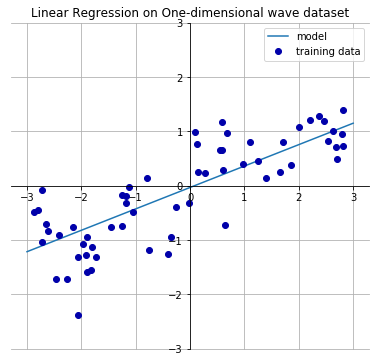
Let's look at an one-dimensional (one input variable) wave dataset which will have a following linear line that best approximates the input features with output values.
From the output below, we see that the slope w[0] of the linear line is around 0.4. The intercept b is close to 0.
import mglearn
import matplotlib.pyplot as plt
import matplotlib

mglearn.plots.plot_linear_regression_wave(); plt.title('Linear Regression on One-dimensional wave dataset')
fig = matplotlib.pyplot.gcf(); fig.set_size_inches(8, 6); plt.show()
Linear models for regression can be characterized as regression models for which the prediction is
- a line for a single input feature (1D),
- a plane when using two features (2D), or
- a hyper‐plane in higher dimensions (that is, when using more features).
There are many different linear models for regression. The difference lies in how the model parameters w and b are learned from the training data, and how model complexity can be controlled. In this post, we will look at the most popular linear models for regression, namely
Linear Regression
Ridge Regression
Lasso
Linear Regression
- Aka ordinary least squares (OLS), is the simplest and most classic linear method.
- Linear Regression finds the best parameters
wandbthat minimises the mean squared error between true output, y and predicted output, h(x) or on the training set. mean squared error (MSE)= sum of squared differences between between the true and prediction values
Linear regression has no parameters to control/tune which makes it easy to use, but it also has no way to control model complexity.
For more details, refer http://scikit-learn.org/stable/modules/linear_model.html#ordinary-least-squares
makewave: 1-D dataset
Let's look at an one-dimensional (one input variable) wave dataset for which we will find a linear line that best approximates the input features with output values.
import mglearn
from sklearn.linear_model import LinearRegression
from sklearn.model_selection import train_test_split
import numpy as np

X,y = mglearn.datasets.make_wave(n_samples=60)
X_train, X_test, y_train, y_test = train_test_split(X,y, random_state=42)

lr = LinearRegression().fit(X_train, y_train)        # Fit the linear regression model on the training data
- The
intercept_attribute learned by theLinearRegression().fit(X_train, y_train)method will always be a single float number. - The
coef_learned is anumpyarray with one entry per input feature.- As the
wavedataset code has only one input feature,coef_only has a single entry.
- As the
print ('--- Slope and intercept learned from the wave training data by Linear Regressor ---')
print ("lr.coef_: {}".format(lr.coef_))              # slope or weight parameter learned from the training data
print ("lr.intercept_: {}".format(lr.intercept_))    # intercept along y-axis learned from the training data
print ('--- Compute the linear line learned to include in the plot ---')
linear_x = np.array([min(X), max(X)])
predicted_y = lr.coef_ * linear_x + lr.intercept_
plt.figure(figsize=(7,5))

plt.plot(X_train,y_train, 'o')                        # plot the training data
plt.plot(X_test,y_test, 'x')                          # plot the test data

plt.plot(linear_x, predicted_y)                       # plot the predicted linear line learned by the LR model

# --- Center the axis tick marks --- #
ax = plt.gca(); plt.ylim([-3,3])
ax.spines['right'].set_color('none'); ax.spines['top'].set_color('none')
ax.xaxis.set_ticks_position('bottom'); ax.spines['bottom'].set_position(('data',0))
ax.yaxis.set_ticks_position('left'); ax.spines['left'].set_position(('data',0))

plt.legend(['training data', 'test data', 'model'])
plt.title('Input data and corresponding linear model')
plt.grid(); plt.show()
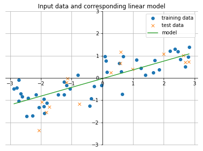
print("Training set score: {:.2f}".format(lr.score(X_train, y_train)))
print("Test set score: {:.2f}".format(lr.score(X_test, y_test)))
An
R2test score of 0.66 is not very good.- We achieved a training score of 0.819 & Test score of 0.834 using KNN with
n=3in previous post for the same dataset.
- We achieved a training score of 0.819 & Test score of 0.834 using KNN with
- However, scores on training and test sets are very close when using Linear Regression.
- This implies we are likely undefitting.
- For 1D dataset, the model is usually very simple and restricted and there's little danger of overfitting.
- However, for higher dimensional datasets (i.e. dataseets with more number of features), linear models become more powerful, and there's more chance of overfitting.
- If we compare the predictions made by straight line with those made by the
KNNin previous post, using a straight line to make predictions seems very restrictive.- It's somewhat unrealistic to assume that our target y is a linear combination of features.
- This gives a skewed perspective when we look at 1D data
- For multi dimensional dataset, linear models can be very powerful.
boston housing: n-D dataset
- Let’s take a look at how
LinearRegressionperforms on a more complex dataset, like theBoston Housing dataset. - This dataset has 506 input samples and 105 derived features (or) variables.
- First, we load the dataset and split it into a training and a test set. Then we build the linear regression model as before:
import mglearn
from sklearn.linear_model import LinearRegression
from sklearn.model_selection import train_test_split
import numpy as np

X,y = mglearn.datasets.load_extended_boston()
X_train, X_test, y_train, y_test = train_test_split(X,y, random_state=0)
print ("Shape of training set: {}".format(X_train.shape))
print ("Shape of test set    : {}".format(X_test.shape))

lr = LinearRegression().fit(X_train, y_train)       # Fit the linear regression model on the training data

print ("\nFirst 5 lr coefficients: {}".format(lr.coef_[:5]), "...")
print ("lr intercept: {}".format(lr.intercept_))
print ("No of lr coefficients learned: {}".format(len(lr.coef_))) # Same as number of input features

print("\nTraining set score: {:.2f}".format(lr.score(X_train, y_train)))
print("Test set score    : {:.2f}".format(lr.score(X_test, y_test)))
From the training and test scores, we find that the prediction is good on training set, but
R2score is worse on the test set.- This discrepancy is a clear sign of overfitting
- So, we should find a model that allow us to control complexity
Ridge regression- Most commonly used alternative to standard linear regression, which we will look into next.
Ridge Regression
- Rigde regression addresses some of the problems of standard Linear Regression (Ordinary Least Squares) by imposing a penalty on the size of the coefficients.
- We want the magnitude of coefficients (weights or slope) to be as small as possible; in other words, all values of
wshould be close to zero.- Intuitively, this means each feature should have as little effect on the outcome (=> having a small slope) while still predicting well.
- This constraint is called as
Regularization
Regularization means explicitly restricting a model to avoid overfitting.
- The ridge regression used here is also known as
L2 regularization, which penalizes the Euclidean length of w
The ridge coefficients minimize the penalized residual sum of squares.

boston housing: n-D dataset
Let's ses how well ridge regression performs on the boston house dataset.
import mglearn
from sklearn.linear_model import Ridge
from sklearn.model_selection import train_test_split
import numpy as np

X,y = mglearn.datasets.load_extended_boston()

X_train, X_test, y_train, y_test = train_test_split(X,y, random_state=0)
print ("Shape of training set: {}".format(X_train.shape))
print ("Shape of test set    : {}".format(X_test.shape))

ridge = Ridge().fit(X_train, y_train)

print("Training set score: {:.2f}".format(ridge.score(X_train, y_train)))
print("Test set score: {:.2f}".format(ridge.score(X_test, y_test)))
- When trained using
linear regression, the training score was0.95whereas test score was0.61. - When trained using
ridge regression, the training score was0.89(lower thanLR) but test score was0.75(higher thanLR).
The results are consitent with our expectation.
- With
linear regression, we were overfitting our training data. Ridgeis a more restricted model, and we are less likely to overfit- A less complex model => worse performance on train set, but better generalization on unknown test set.
alpha
The Ridge model makes a trade-off between the model simplicity (near-zero `w` coefficients) and its performance on training set.
- The tradeoff can be specified by the us, using the
alphaparameter (called asRegularization strength) - When
alphaparameter is not specified as in previous case, it uses default value ofalpha=1.0, which have to be optimized for each dataset.
Larger values specify stronger regularization (by forcing the coefficients w to move toward zero), which decreases the training set performance but might help generalization
training_score = []
test_score = []
alpha_settings = [0.001, 0.003, 0.01, 0.03, 0.1, 0.3, 1.0, 3, 10, 30, 100]
for alpha in alpha_settings:
    ridge = Ridge(alpha=alpha).fit(X_train, y_train)
    training_score.append(ridge.score(X_train, y_train))
    test_score.append(ridge.score(X_test, y_test))
    print("alpha: {:8.4f} | Training score: {:.2f} | Test score: {:.2f}".format(
           alpha, ridge.score(X_train, y_train), ridge.score(X_test, y_test)))
import matplotlib.pyplot as plt
import matplotlib

plt.figure(figsize=(6,4))

plt.semilogx(alpha_settings, training_score, '-.', label="training R^2 score")
plt.plot(alpha_settings, test_score, '-.', label="test R^2 accuracy")
plt.ylabel("R^2 score")
plt.xlabel("alpha (in log scale)")
plt.title("Comparison of training and test R^2 score as a function of alpha\n")
plt.legend(); plt.grid()

print ('--- Based on test set/ generalization ---\n')

index = test_score.index(max(test_score))
print ('Best alpha  = {} | Training score = {:0.3f} | Test score = {:0.3f}'.
       format(alpha_settings[index], training_score[index], test_score[index]))

plt.plot(alpha_settings[index], training_score[index], 'x')
plt.plot(alpha_settings[index], test_score[index], 'x')

index = test_score.index(min(test_score))
print ('Worst alpha = {} | Training score = {:0.3f} | Test score = {:0.3f}'.
       format(alpha_settings[index], training_score[index], test_score[index]))

plt.show()
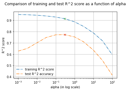
From the above plot, we see how the alpha corresponds to the model complexity.
- It's evident that decreasing
alphafrom 100 to 0.1 allows the coefficients to be less restricted (we fix underfitting issue). - However if the
alphavalue is set too low (below 0.1), coefficients are barely restricted (we start facing overfitting issue) as the penalty for cost function is very low.- Think, what happens when α is set to a very small value (close to 0).

- We end up with a ridge model that is similar to
Linear Regression.
- Think, what happens when α is set to a very small value (close to 0).
alpha = 0.1 or 0.3 seems to work well. We will discuss more about parameter optimization in later topics.
# compare the different models (KNN with linear and ridge regression) on the multi dimensional `boston` dataset
from sklearn.neighbors import KNeighborsRegressor

training_score = []
test_score = []
# try n_neighbors from 1 to 20
neighbors_settings = range(1, 21)

for n_neighbors in neighbors_settings:
    # intialize the knn model parameters
    knn = KNeighborsRegressor(n_neighbors=n_neighbors)
    # build/ train the model
    knn.fit(X_train, y_train)
    # save training set accuracy
    training_score.append(knn.score(X_train, y_train))
    # save test set (generalization) accuracy
    test_score.append(knn.score(X_test, y_test))

plt.figure(figsize=(6,4))
plt.plot(neighbors_settings, training_score, label="training R^2 score")
plt.plot(neighbors_settings, test_score, '--', label="test R^2 accuracy")
plt.ylabel("Accuracy")
plt.xlabel("n_neighbors")
plt.title("Comparison of training and test R^2 score as a function of n_neighbors [in KNN]\n")
plt.legend()
plt.show()

print ('--- Based on test set/ generalization ---\n')

index = test_score.index(max(test_score))
print ('Best n_neighour  = {} | Training score = {:0.3f} | Test score = {:0.3f}'.
       format(neighbors_settings[index], training_score[index], test_score[index]))

index = test_score.index(min(test_score))
print ('Worst n_neighour = {} | Training score = {:0.3f} | Test score = {:0.3f}'.
       format(neighbors_settings[index], training_score[index], test_score[index]))
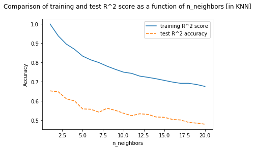
- Best test score using
Linear Regression = 0.610 - Best test score using
Ridge Regression = 0.773 - Best test score using
K-NearestNeighbours = 0.652
alpha - Qualitative insight
We can also get a more qualitative insight into how alpha parameter changes the model by inspecting the coef_ (slope or weight) attribute of models.
ridge = Ridge(alpha=1).fit(X_train, y_train)
ridge10 = Ridge(alpha=10).fit(X_train, y_train)
ridge01 = Ridge(alpha=0.1).fit(X_train, y_train)
lr = LinearRegression().fit(X_train, y_train)

plt.figure(figsize=(16,6))
plt.title('Comparing coefcient magnitudes for ridge regression with different values of alpha and for linear regression')
plt.plot(ridge.coef_, 's', label="Ridge alpha=1")
plt.plot(ridge10.coef_, '^', label="Ridge alpha=10")
plt.plot(ridge01.coef_, 'v', label="Ridge alpha=0.1")
plt.plot(lr.coef_, 'o', label="LinearRegression")
plt.xlabel("Coefficient index")
plt.ylabel("Coefficient magnitude")
plt.hlines(0, 0, len(lr.coef_))
plt.xlim(0,50)
plt.ylim(-25,25)
plt.legend()
plt.show()

print ("No of features = No of coefficients = {}".format(len(lr.coef_)))
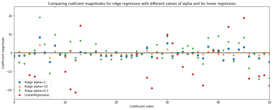
A higher alpha means a more restricted model (more penalty), so we execpt the coef_ (weights) to have smaller magnitude for a higher value of alpha.
This is confirmed by the above plot. Here,
x-axisspans over 104 data points, but only first 50 data point are shown. It corresponds to thecoeff_orweightofnth feature/ dimensiony-axisshows the numeric (magnitude) values of the corresponding values of the coefficients.■ Coefficients of Ridge model with alpha=1. Here, the coefficients are somewhat larger than range of -3 to 3
▲ Coefficients of Ridge model with alpha=10. Here, the coefficients are mostly between -3 to 3
▼ Coefficients of Ridge model with alpha=0.1. Here, the coefficients have large magnitude
● Coefficients of Linear model (no alpha parameter involved). Here, the coefficients are so large that many of them are outside the chart range
Training size - insight
Another way to understand the effect of regularization is to fix alpha but vary the size of training data.
In the figure below, the boston housing dataset is subsampled & evaluated on LinearRegression and Ridge(alpha=1) with training subsets of increasing size.
plt.figure(figsize=(10,6))
mglearn.plots.plot_ridge_n_samples()
plt.title('Learning curves for ridge regression and linear regression \n on Boston housing dataset', y=1.2)
plt.grid()
plt.ylim([-0.5,1.02])
plt.show()
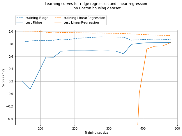
From the above learning curve, we can deduce that
- Training score is higher than test score for different training set size, for both linear and ridge regression.
- As ridge is regularized (as weights are constrained), the training score of ridge is always lower than linear regression.
- However, the test score for ridge is better, especially for smaller training dataset.
As more and more data becomes available for training the model, both models improve, and linear regression catches up with ridge. The lesson here is that with enough training data, regularization becomes less important. Another interesting aspect is the decrease of training set preformance when more data is added. This implies that, with more data, it becomes harder for the model to overfit or memorize the data crudely.
Lasso
An alternative to
Ridgefor regularizing and to restrict the weight/ slope coefficients close to zero, but in a slightly different way.The lasso regression is also known as
L1 regularization, penalizes the sum of absolute value of thewThe ridge regression is also known as
L2 regularization, penalizes the Euclidean length ofw
The consequence of L1 regularization is that when using lasso, some coefficients are exactly zero
This can be seen as automatic feature selection, where having some coefficients as 0 reveals the most important features of the model, thereby making it easier to interpret it
boston housing: n-D dataset
import mglearn
from sklearn.linear_model import Lasso
from sklearn.model_selection import train_test_split
import numpy as np

X,y = mglearn.datasets.load_extended_boston()
X_train, X_test, y_train, y_test = train_test_split(X,y, random_state=0)
print ("Shape of training set: {}".format(X_train.shape))
print ("Shape of test set    : {}".format(X_test.shape))

lasso = Lasso().fit(X_train, y_train)
print ("\n" + 'Lasso details:', lasso)
print ("\nNumber of features used: {} out of {}".format(np.sum(lasso.coef_ != 0), X.shape[1]))

print("Training set score: {:.2f}".format(lasso.score(X_train, y_train)))
print("Test set score: {:.2f}".format(lasso.score(X_test, y_test)))
alpha
- We can see that Lasso does quite badly on both training (
0.29) and testing (0.21) whereas Ridge scored0.77on test set. - A low training and test score indicates underfitting and it's obvious that the model only used
4out of104input features - Similar to
Ridge, we can control the regularization strength usingalphaparameter. - To resovle underfitting issue, let's reduce the
alphafromdefault value (1.0)to0.01, thereby reducing the regularization strength.
lasso = Lasso(alpha=.01, max_iter=100000).fit(X_train, y_train)
print ("\n" + 'Lasso details:', lasso)
print ("\nNumber of features used: {} out of {}".format(np.sum(lasso.coef_ != 0), X.shape[1]))

print("Training set score: {:.2f}".format(lasso.score(X_train, y_train)))
print("Test set score: {:.2f}".format(lasso.score(X_test, y_test)))
- It's evident that lower
alphaallows us to fit a more complex model, thereby improving the score. - The performance on test data is
0.77and is slightly better thanRidgeas we are using only 33 out of 104 features. - If we set the
alphatoo low, we again remove the effect of regularization and end up overfitting, similar toLinearRegression.
lasso = Lasso(alpha=.0001, max_iter=100000).fit(X_train, y_train)
print ("\n" + 'Lasso details:', lasso)
print ("\nNumber of features used: {} out of {}".format(np.sum(lasso.coef_ != 0), X.shape[1]))

print("Training set score: {:.2f}".format(lasso.score(X_train, y_train)))
print("Test set score: {:.2f}".format(lasso.score(X_test, y_test)))
- It's evident that a very low
alpha(close to 0) causes overfitting, thereby failing to generalize well on test set.
alpha - Qualitative insight
lasso1 = Lasso(alpha=1).fit(X_train, y_train)
lasso0_01 = Lasso(alpha=0.01, max_iter=100000).fit(X_train, y_train)
lasso0_0001 = Lasso(alpha=0.0001, max_iter=100000).fit(X_train, y_train)
ridge0_1= Ridge(alpha=0.1).fit(X_train, y_train)

plt.figure(figsize=(16,6))
plt.title('Comparing coefcient magnitudes for lasso regression with different values of alpha and for ridge regression')
plt.plot(lasso1.coef_, 's', label="Lasso alpha=1")
plt.plot(lasso0_01.coef_, '^', label="Lasso alpha=0.01")
plt.plot(lasso0_0001.coef_, 'v', label="Lasso alpha=0.0001")
plt.plot(ridge0_1.coef_, 'o', label="Ridge alpha=0.1")
plt.xlabel("Coefficient index")
plt.ylabel("Coefficient magnitude")
plt.hlines(0, 0, len(ridge0_1.coef_))
plt.xlim(0,50)
plt.ylim(-25,25)
plt.legend()
plt.show()

print ("No of features used by Lasso(alpha=1)     = {}".format(np.sum(lasso1.coef_ != 0)))
print ("No of features used by Lasso(alpha=0.01)  = {}".format(np.sum(lasso0_01.coef_ != 0)))
print ("No of features used by Lasso(alpha=0.0001 = {}".format(np.sum(lasso0_0001.coef_ != 0)))
print ("No of features used by Ridge(alpha=0.1)   = {}".format(len(ridge0_1.coef_)))
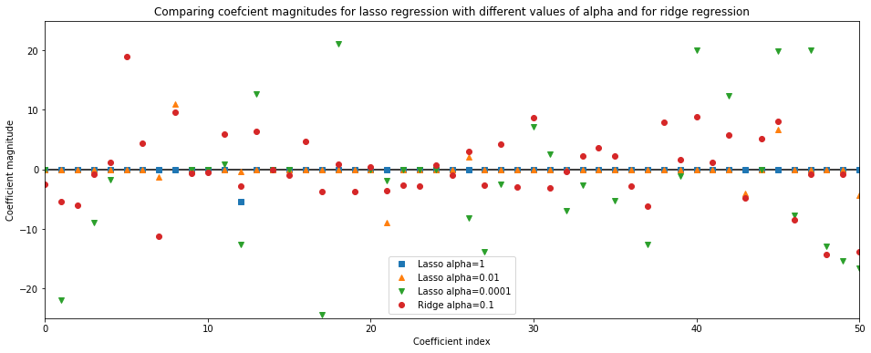
A higher alpha means a more restricted model (more penalty), so we execpt a lot of losso coef_ (weights) to have zero magnitude for a higher value of alpha.
This is confirmed by the above plot. Here,
x-axisspans over 104 data points, but only first 50 data point are shown. It corresponds to thecoeff_orweightofnth feature/ dimensiony-axisshows the numeric (magnitude) values of the corresponding values of the coefficients.■ Coefficients of
Losso model with alpha=1: Here, the majority of the coefficients are zero and the remaining 4 features are also small in magnitude▲ Coefficients of
Losso model with alpha=0.01: Here, most of the features are still zero, but the remaining 33 features are slightly less restricted than when alpha=1▼ Coefficients of
Losso model with alpha=0.0001: Heremodel is slightly unregularized, woith most coefficients non-zero and large magnitude● Coefficients of
Ridge model with alpha=0.1: Here, all the coefficients are non-zero though the test results are similar to Lasso model with alpha=0.01
Miscallaneous
Additional Datasets
Dataset 1: 1-D
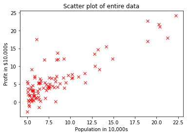
You are the CEO of a restaurant franchise and are considering different cities for opening a new outlet. The chain already has trucks in various cities and you have data for profits and population from cities.
You would like to use this data to help you select which city to expand next based solely on the city population.
- The first column is the population of city and
- the second column is the profit of a good truck in that city. The -ve value for profit indicates a loss
# This block of code downloads the data file from GitHub incase if it doesn't exist in the computer
import urllib
import os

url = '''https://prasanth-ntu.github.io/html/ML-Course/Intro-to-ML-with-Python/data/ex1data1.txt'''

path =  os.path.join(url.split("/")[-2], url.split("/")[-1])

if not os.path.exists(path):
    path_out, message = urllib.request.urlretrieve(url, path)
    print ("File downloaded to:", path)
else:
    print ("File already exists:", path)
import pandas as pd
data = pd.read_csv(path, header=None, names=['Population in 10,000s', 'Profit in $10,000s'])
data.head() # displays the first 5 rows
data.describe() # displays the basic stats of each column
import numpy as np

fname = path
data = np.genfromtxt(fname, delimiter=',')
print ("Size of dataset:", data.shape)

X = data[:,0:1]   # input feature - city population
y = data[:,-1]    # output  - profit

plt.plot(X,y, 'rx')
plt.xlabel('Population in 10,000s')
plt.ylabel('Profit in $10,000s')
plt.title('Scatter plot of entire data')
plt.show()
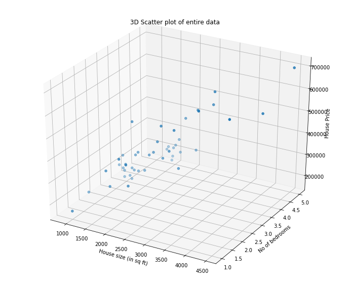
Dataset 2: 2-D
Suppose we are selling our hoeu and we want to know what a good market price would be. One way to do this is to first collect information on recent houses sold in the neighourhood and make a model of housing prices.
- The first column in the size of the house (in sq feet)
- the second column in the number of bedrooms
- the third column is the price of the house
# This block of code downloads the data file from GitHub incase if it doesn't exist in the computer
import urllib
import os

url = '''https://prasanth-ntu.github.io/html/ML-Course/Intro-to-ML-with-Python/data/ex1data2.txt'''

path =  os.path.join(url.split("/")[-2], url.split("/")[-1])

if not os.path.exists(path):
    path_out, message = urllib.request.urlretrieve(url, path)
    print ("File downloaded to:", path)
else:
    print ("File already exists:", path)
import pandas as pd
data = pd.read_csv(path, header=None, names=['House size (in sq ft)','No of bedrooms','House price'])
data.head() # displays the first 5 rows
data.describe() # displays the basic stats of each column
import numpy as np

fname = path
data = np.genfromtxt(fname, delimiter=',')
print ("Size of entire dataset:", data.shape)

X = data[:,0:2]   # input features
y = data[:,-1]    # output  -

from mpl_toolkits.mplot3d import Axes3D
fig = plt.figure(figsize=(12,10))
ax = fig.add_subplot(111, projection='3d')
ax.scatter(X[:,0], X[:,1], y)

ax.set_xlabel('House size (in sq ft)')
ax.set_ylabel('No of bedrooms')
ax.set_zlabel('House Price');

plt.title("3D Scatter plot of entire data")
plt.show()
Dataset 3: n-D
The code below will generate some sparse data to play with.
To generate more features per input sample, change the n_features variable and to generate more data samples, increase the n_samples variable in the code below.
n_samples, n_features = 50, 200

import numpy as np
import matplotlib.pyplot as plt

from sklearn.metrics import r2_score

# #############################################################################
# Generate some sparse data to play with
np.random.seed(42)

X = np.random.randn(n_samples, n_features)
coef = 3 * np.random.randn(n_features)
inds = np.arange(n_features)
np.random.shuffle(inds)
coef[inds[10:]] = 0  # sparsify coef  => Makes most of the coef as zero
y = np.dot(X, coef)

# add noise
y += 0.01 * np.random.normal(size=n_samples)

print ("Dataset size:", X.shape, y.shape)
ElasticNet
ElasticNet
- A linear regresion model that combines the penalaties of
LassoandRidge - This combination works best in practice, though at the price of haign two parameters to adjust
- one for L1 regularization
- one for L2 regularization
Refer http://scikit-learn.org/stable/modules/linear_model.html#elastic-net for more details on it as it's out of scope for this post.
import mglearn
from sklearn.linear_model import ElasticNet
from sklearn.model_selection import train_test_split
import numpy as np

X,y = mglearn.datasets.load_extended_boston()
X_train, X_test, y_train, y_test = train_test_split(X,y, random_state=0)
print ("Shape of training set: {}".format(X_train.shape))
print ("Shape of test set    : {}".format(X_test.shape))
training_score_list = []
test_score_list = []
best_test_score = None
best_alpha = 0; best_l1_ratio = 0

alpha_settings = [0.001, 0.003, 0.01, 0.03, 0.1]
l1_ratio_setting =  [0.1,0.2,0.3,0.4,0.5,0.6,0.7,0.8,0.9,1]
for alpha in alpha_settings:
    for l1_ratio in l1_ratio_setting:
        elastic = ElasticNet(alpha=alpha,l1_ratio=l1_ratio, max_iter=100000, random_state=42).fit(X_train, y_train)
        train_score, test_score = elastic.score(X_train, y_train), elastic.score(X_test, y_test)
        training_score_list.append(train_score)
        test_score_list.append(test_score)
        print("alpha: {:8.4f} | l1_ratio: {:8.4f} | Training score: {:.4f} | Test score: {:.4f}".format(alpha, l1_ratio, train_score, test_score))

        if best_test_score is None or best_test_score < test_score:
            best_test_score = test_score
            best_alpha = alpha
            best_l1_ratio = l1_ratio

print ("\n\n----------------- BEST on TEST set----------------")
elastic = ElasticNet(alpha=alpha,l1_ratio=l1_ratio, max_iter=100000, random_state=42).fit(X_train, y_train)
print ("Coefficients of the elastic model:", elastic.coef_)
Summary
We have covered about 3 most popular linear models for regression, namely
Linear RegressionRidge RegressionLasso
General Practice
linear regressionis where people start with as it doesn't involve any tuning of parameters, likealpha. However, the LR model might easily overfit on the training set and fail to generalize on test set.ridge regressionis usually the first choice when compared toLasso, especailly when we have fewer features
When is Lasso better?
- If we have large number of input features and expect only few of them to be important,
Lassois a better choice - If we would like to have a model that is easy to interpret,
Lassois better as it will select only a subset of features.
Now that we have covered Linear models for regression, let's explore Linear models for Classification in the next post.